Azimuth Survey

Introduction

This exercise gave us the chance to learn a new method of field survey. This method is actually very old and requires very little technology.  The method, called Azimuth survey, does just what the name implies.  It uses a fixed location, the distance to a new location, and the direction toward the new location to attain the coordinates of the new location.  You can go as low tech as a compass and measuring tape all the way up to fancy gadgets that use lasers and radio signals to determine the distance and azimuth.  The benefit of learning this technique is that when all the electronics break down, we still have the ability to collect rudimentary points with the minimum of equipment.

For our survey we used the LTI TruPulse laser rangefinder.  The TruPulse is a handheld (but can be tripod mounted) device that sends a laser beam to the target you designate by looking through the eye sight.  The beam bounces back and is measured to give the distance.  This distance is displayed in the eye piece and measures down to .0 meters.  The TruPulse also has a compass built in that allows the user to collect the azimuth of a target in the same manner as the distance. The azimuth is collected in 360.0 degree readings.  This model has several other features that we did not use, including Slope distance, Vertical distance, and Inclination.

Study Area

As part of our preparation for this exercise we were given a demonstration and a brief test period with the TruPulse rangefinder to help familiarize ourselves with the device.  Our test location was the courtyard of Phillips hall on the University of Wisconsin – Eau Claire campus.  This location is an open green space contains several raised garden beds, as well as a few small trees and picnic tables.  Working in two-man teams, each group collected a few points with the device and recorded them on paper.  Once this was complete, we went back to the lab and entered the data into a spreadsheet. This process will be discussed more the methods section. 

As part of our survey we were told to select a location and to collect 100 data points there, as well as some attribute associated with those points.  Our group chose Owen Park as our location with the intention of surveying the location of trees in the park.  We chose this location as it would provide a good line of sight between the start point and the target points.  We decided to use tree height in meters as our attribute and chose to use three categories to be estimated for each tree point: “under 5”, “5-10”, and “over 10”. 

One thing not mentioned yet is the importance of the start point.  The data we are collecting is implicit data, meaning that each point is relative to the point of origin.  There are a few ways to collect the start point.  A GPS unit can be used to collect a point, or using some georeferenced aerial or satellite imagery to pinpoint the location.  We chose the latter; which for the first point was the inside corner of the sidewalk on the east side of first avenue, and the second point we visually aligned ourselves with the south edge of the sidewalk on Niagara st as our X axis and the same sidewalk on 1^st Ave as the Y axis.  These landmarks were easy to find later.  We also opted to use a tablet computer to enter our data directly into a spreadsheet, this was a little clunky, but in the end it saved a good bit of time.

Methods

                Preparation list:

(low tech) Compass, measuring rope, notebook and pencil.
(high tech)  Rangefinder, GPS, tablet computer.
Optional tripod for Rangefinder is a great plus.
Location with desired data.
Clear weather.  (weather should not effect a rangefinder, but it could make you miserable)
Data fields to collect: Number, Distance, Azimuth, Attribute.  Start point coordinates.

Once you are at your location you must pick you start point.  It is important to move as little as possible once you have begun collecting data, since each point is collected from the start, and if the start keeps moving you will have a lot more error.  Make notes of your start location if you do not have a GPS, it is crucial to have your start point as accurate as possible.

If using a rangefinder, sight up your target and hit the collect button.  When you have your distance and azimuth recorded sight of the next target.  Once you have the desired number of points you are finished in the field.

Once in the lab you need to enter the data to a spreadsheet if it is not already.  Here is where you will need to add you start locations.  In your spreadsheet select a new column for your longitude (X) and another for your Latitude (Y).  Enter your coordinates in the cell then drag down the corner to populate all the cells in that column that used that start point.  If you did not have a GPS unit to find your start coordinates, you will need to use an online source like Google Earth, or any of the others.  Be warned that Google Earth uses Degree Minutes and seconds, you will need to convert this to decimal degrees before you import.  There are many online converters available.  If you do not convert to decimal degrees, your data may end up in the next county, as ours did.  Another thing to keep in mind is that when moving west of the prime meridian, the number become negative, otherwise your point will end up on the opposite side of the world. Your table should look like table 1.

 

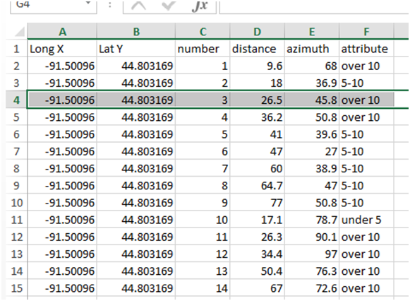Table 1.  This table is a sample of our data that we collected.  It shows the corrected X and Y coordinates, point number, distance, azimuth, and a specific attribute.  In our case we collected trees and estimated their height in meters divided into three categories: Under 5m, 5-10m, and over 10m.

You will need to have a geodatabase ready to go for your project at this point.  Once you have your data you will need to import it into your geodatabase, you cannot just add it to your geodatabase.  Trust me, if you don’t import it, you will spend many hours failing at the next steps.

To import the spreadsheet, right click on the geodatabase>import>table(single) as seen in figure 1.  This opens up the dialogue seen in figure 2.  You want to click the folder on the right of the input rows, this will take you to the next window where you select the table you want, then select the proper sheet.  Then you will need to name your import output.

Figure 1. Showing the right-click menu path to import a single table into your Geodatabase.  This one simple trick will save you hours in the lab.  But really, you can't run the next tools if you don't import the data. Figure 2 shows the next steps.

Figure 2. This is the dialogue box that opens from the menu shown in figure 1.  Just select your spreadsheet as the input, then designate the location you want the output saved in, and press OK.  This will allow you to run the required tools on the table.

Once the table is imported you will add the data to ArcMap. Click the + button in the top tool bar (figure 3).  Since this is not spatial data yet, it will not show up in the Table of Content – Drawing Order list, click the list by sources button.  

Figure 3. This shows the dialogue box used to add data to your .mxd. First click the + sign just below selection, then click on your table in the dialogue box.  Your table will now be in your table of contents window, just select the list by source tab (second from left) since the table has no spatial reference points and is not yet drawn. 

Now you will the Bearing Distance to Line tool, this uses the start coordinates, the distance, and azimuth to create a line the length of your distance field, and in the direction of your azimuth from your start point.  In the dialogue box the tool opens you first select you table, then select your X as the X field; your Y as the Y field; your distance as the distance field; and you azimuth as the bearing field.  You should also use your number column in the ID field to join your table to later.  Click OK and the tool will run (figure 4).

Figure 4. On the left is the Bearing Distance to Line tool dialogue box.  To use the tool select your table as the input, then choose your X to the X field, ect. ect. Not shown is the optional ID field. Select the number field, this will let you join your feature to your table later and let you symbolize your attributes.
On the right is the ArcToolbox showing the path to find the Bearing Distance to Line tool.

Next you will use the Feature Vertices to Point tool (figure 5). See figure 6 for tool location. Simply select your line feature as your input, name your output and click OK.  You will then have a point created at the end of each line.  The down side of this is that there will now be a large number of points on your start point.  You can click the editor toolbar and start an edit session, then open the table and delete the excess points. 

Figure 5. The Feature Vertices to Points tool takes the end points of the lines created by the Bearing Distance to Lines tool and creates points. The downside is that there are now as many points at your start location as there are everywhere else. Pretty straightforward, select the lines that you just created in the input, and choose where the output is saved. See figure 6 for tool location. 

Figure 6.  This shows the ArcToolbox path tothe Feature Vertices to Points tool. Data management Tools > Features > Feature Vertices to Points.

The last thing to do is to join your table to the points feature.  Right click your feature>joins and relates>join…  (figure 7). In the join dialogue box select “number” as the join field.  The same should apear in field 3, then click OK(figure 8).  Your table is now joined and you should be able to symbolize your data by attribute as desired.

Figure 7. This is the right-click menu path used to join your
points feature and your data table.

Figure 8. This is the Join Data dialogue box.
Box 1 lets you choose the field that you are
joining, box 2 is covered, but it shows you
your table options, box 3 is the field in the table
that your join will be based on. It should
 self-populate once you pick your table.

Results

The results of the data collection are seen below in figure 8.  This map shows the data points, as well as the lines.  Figure 9 shows a close up of the start points, in it you can see that the points are shifted about a meter west of where they should be.  One possible reason for this shift is the imprecise nature of finding the origin points in Google Earth.  Another reason could be the slight differences in the projections and georeferencing of the base images.

Figure 9. This is the final product map. It shows the tree height attribute that was collected. Figure 10 shows a close-up of the start point to give a better view of how far off they are.

It is mostly difficult to tell how closely the points line up with the trees since many is clustered together.  I would say most appear to be about as far off as the start points.  Table 10 shows a close up of the start points.  The first location we collected from is on the bottom side on the corner of the sidewalk.  The point is about a meter to the left of where we stood in the real world. Other causes of error in this would be the size of the tree.  If the tree is very small it is possible to miss the tree and hit the background several meters away.  We were very conscious of staying in the same position the whole time, but it wouldn't take much movement to noticeably increase the error.

Figure 10. This is a close-up of the start points. The first collection point is at the bottom, about a meter to the left of where we stood in the real world.  The second point is also about a meter to the left of where we stood.  We tried to be very careful when picking our locations. The first lined up with the corner of the sidewalk, while the second was lined up with the sidewalk across the street.

Conclusion

This exercise taught us the Azimuth survey method.  We learned the high tech and low tech way of conducting this type of survey.  Azimuth survey uses the coordinates of a known location combined with the distance and azimuth to a new location to acquire the coordinates of that new location.  This can be done with as little as a compass and as high tech as rangefinders and survey stations.   This is another great tool to have in the old cranial tool box for when the electronics gods take the day off. 

 The exercise had a good combination of field and lab work.  While the collection could lean toward busy work, it forced us to get to know our equipment better than if we had gone out and gotten 10 or 20 points.  It also helped to consider the spatial surroundings better to look for ways to increase our efficiency.  100 points also gives a much better impression of how accurate, or inaccurate this method of survey can be.